 EN
EN 中文
中文 ES
ES RU
RU FR
FR PT
PT AR
AR DE
DEHow 3D LiDAR Measures Stockpile Volume: From Point Cloud to Tonnage
Measuring an open stockpile of coal, ore, or aggregate by hand has always been a compromise between effort and accuracy. Manual surveys interrupt operations, drone flights depend on weather and crew availability, and load-count estimates drift as material is added and drawn from many points. A fixed 3D scanner removes that compromise by continuously rebuilding the pile surface as a measurable geometric object. Understanding lidar stockpile volume measurement means following one chain of steps: scanning the surface into a point cloud, aligning it to a known ground reference, computing the enclosed volume, and converting that volume to tonnage using an assumed density. Each step has its own error sources, and knowing where they sit is the difference between a number you can plan around and one you merely hope is right.
This article walks through that chain for the Volivue 3D LiDAR Stockpile Inventory System, a fixed laser scanner that builds the surface point by point rather than relying on a single distance reading. The goal is to explain the physics and geometry plainly, so engineers and plant managers can judge what the output represents and what it does not.
Scanning the surface into a point cloud
A fixed 3D LiDAR scanner emits laser pulses and measures the time each pulse takes to return from a surface. With a known beam direction and a measured range, every return becomes a single 3D coordinate relative to the scanner. Sweep the beam across the stockpile and you accumulate thousands to millions of these coordinates: a point cloud that traces the visible shape of the pile.
Range depends on the model, the material’s reflectivity, and airborne conditions. Effective range is typically 0.5 to 100 m, and that figure is model-dependent. Dust, steam, and low-reflectivity surfaces shorten usable range and reduce the number of clean returns, which is why scanner placement and environmental review matter as much as the raw specification. A point that never returns leaves a gap in the surface, and gaps are where volume error begins.
The density of points across the surface is what makes a 3D scan different from a single-point level reading. Instead of inferring a whole pile from one measurement, the system samples the actual contour, capturing peaks, valleys, draw cones, and irregular edges that a single reading cannot see. For closed silos where the surface is not optically accessible, mass-based methods such as patch-mount weighing or 80 GHz silo radar are the better fit; open stockpiles are exactly where surface scanning earns its place.
Aligning the cloud to a ground-plane reference
A point cloud on its own is just a shell of coordinates. To turn it into a volume you need to know what the pile sits on. The system aligns each scan to a known ground baseline, the floor or pad surface established when the installation is commissioned. That reference defines the zero-height plane beneath the material.
Alignment matters because the scanner sees only the top surface of the pile. The volume of interest is the space between the scanned surface above and the known ground plane below. If the reference is captured accurately at commissioning and the floor does not move, every later scan can be compared against the same datum, so changes in the surface translate directly into changes in stored volume. This is also what allows the system to track a pile that grows and shrinks throughout the day without re-surveying the ground each time.
In multi-region layouts, the floor is partitioned into separate measurement zones, up to 32 zones in the planned configuration, each with its own footprint and reference. Partitioning lets one installation report several material piles or bays independently rather than collapsing everything into a single aggregate number.
From point cloud to volume: the geometry
With the surface aligned to the ground plane, volume becomes a geometry problem. The point cloud is converted into a continuous surface model, and the system integrates the height of that surface over the measured footprint. Conceptually, the footprint is divided into many small cells; for each cell the height above the ground plane is taken from the surface model, and the cell volume is its area multiplied by that height. Summing across all cells yields the enclosed volume between the pile surface and the floor.
The accuracy of this integration depends on how completely and densely the surface was sampled. Where points are plentiful, the surface model closely follows the real contour. Where the scan was sparse or occluded, the model has to interpolate across the gap, and any deviation between the assumed and the true surface in that region adds to volume error. Under field-calibrated conditions, volume accuracy is typically in the 1 to 3 percent range. That figure is realistic for a well-placed scanner on a cooperative material; it is not a fixed guarantee, and it degrades when coverage degrades.
This is why the geometry step cannot be separated from the scanning step. A clean, well-covered point cloud makes the volume calculation almost mechanical. A point cloud full of shadows forces the math to guess, and the percentage error climbs accordingly.
Converting volume to tonnage with density
Volume answers “how much space does the material occupy,” but operations and ERP systems usually want “how many tonnes.” The bridge is bulk density: tonnage equals measured volume multiplied by an assumed density value for the material.
That word “assumed” carries weight. Bulk density for materials such as coal, ore, aggregate, cement raw meal, grain, biomass, and solid waste is not a single constant. It varies with moisture, particle size, compaction, and how recently the material was placed. A freshly tipped pile is looser than one that has settled and consolidated under its own weight. Because the system applies a density value you supply, the tonnage figure is only as good as that value. The volume measurement can be well within its 1 to 3 percent band while the tonnage carries additional uncertainty purely from density assumptions.
The practical implication is to treat volume and tonnage as two separate accuracy questions. Volume is what the scanner and geometry deliver. Tonnage is volume plus a material model you maintain. For materials whose density is stable and well characterized, the two stay close. For variable or moisture-sensitive materials, periodic density checks keep the tonnage honest. Keeping the density assumption explicit, rather than buried, is what lets a team reconcile scanned tonnage against scale tickets when they diverge.
Where the accuracy really comes from
Two factors dominate real-world performance: field calibration and occlusion.
Field calibration ties the system’s geometry to the actual installation. The ground reference, the scanner’s mounting position and orientation, and the measurement footprint are all established on site. Volivue’s typical 1 to 3 percent volume accuracy is stated for post-calibration conditions for exactly this reason; an uncalibrated or shifted installation will not hold that figure. Calibration is not a one-time formality if the mounting or the floor changes over time.
Occlusion is the structural limit of any line-of-sight method. The scanner can only measure surfaces it can see. Tall peaks cast shadows over the material behind them, structural members block portions of the footprint, and material against a wall may be partly hidden from a given vantage point. Mounting options, on the roof, on a gantry, on a mast, or on a wall, exist precisely so the field of view can be optimized for each site, and every installation should include an FOV and occlusion review before it is fixed in place. Where a single scanner cannot see the whole footprint, the multi-zone approach and considered placement reduce the shadowed area that the geometry would otherwise have to interpolate across.
The honest summary is that 3D LiDAR gives a repeatable, traceable volume measurement whose accuracy is governed by coverage and calibration, then layers a density assumption on top to reach tonnage. Treat the output that way and it becomes a dependable basis for inventory reconciliation, production planning, and reorder decisions. Outputs are delivered through OPC UA, REST API, MQTT, CSV, or direct database export, so the measured volume and computed tonnage flow into the systems your team already uses. To discuss whether your site geometry and material suit fixed surface scanning, request a site review or explore the full 3D LiDAR Stockpile Inventory System.
Related reading: for more on stockpile LiDAR principles and how to choose between surface scanning and mass-based methods, browse the Technical Insights library.